

Intro & Lit Review
Predicting the NBA draft is always difficult. Should you draft a player on college statistics, NCAA tournament performance, combine results, potential, or a combination of all of these? The goal of this project is to come up with a model to help management of an NBA team determine how they should draft NBA players. This problem about who to draft has always been difficult to judge. Some teams tend to draft more on college performance and some teams tend to draft more on potential. Another factor is also level of competition on the college level. Some players in smaller colleges may have better stats just because they play against competition that is not as good. Our dataset came from the official website of the NCAA(NCAA.org -The Official Site of the NCAA, 2018). We looked at years 2011-2014 as our training set and 2015 as our test set. If we can create a successful model this will help management know when they should draft players. The purpose of this study is to see if we can use college stats of past draft picks to help our front office pick players for the upcoming draft.
Methods
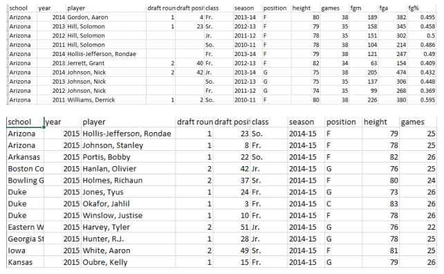
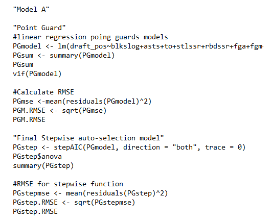
We ran two different models. The first model would ignore all seasons for players who were not drafted in that particular year. For example, we would ignore the first three season for a college senior and focus solely on his stats for his final year of college, which was when he was drafted into the NBA. The assumption of this model that we studied is that only the final season of a player’s college career would have any bearing on how that player was drafted. This model is referred to as “model A.” The second model would combine all the stats for each player’s college career and use his per-game statistics to see if a model based on his full body of work in college would be more representative of how that player would be drafted. We refer to this as “model B.”
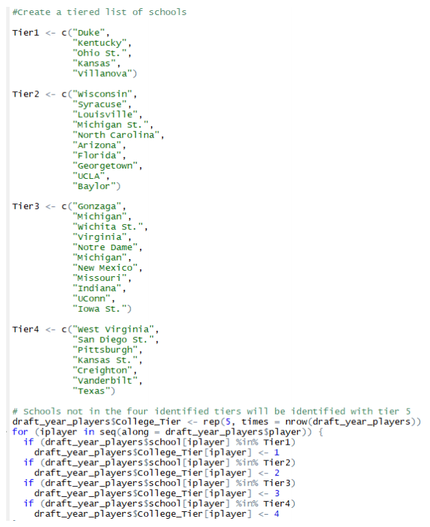
We decided to make a tiered structure of NCAA basketball programs meant to provide more draft stock to players at powerhouse schools such as Kentucky and Duke. Our data examined player stats from 2011-2015, so we conducted a study using the website www.collegepollarchive.com of all AP Top 25 polls over that time frame. In considering what tier to place schools in, the number of appearances in the top 25, average rank, highest rank, and number of appearances in the top 10 were used to identify the most successful basketball programs of that time. The study resulted in 33 schools being identified and divided into four separate tiers. Any school not specifically identified in these tiers were placed into a fifth tier.
A series of box plots were created to determine if the data would need to be further parsed into subsets. We started by examining box plots of statistics by position for each of the two models we were building (samples below)
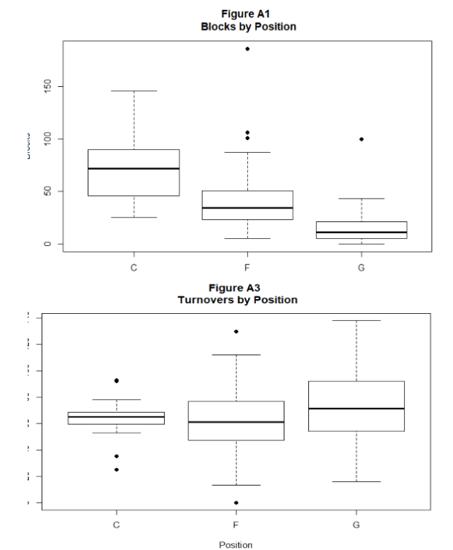
It comes as no surprise that numerous statistics were very different based on the position played. For example, centers would have more blocks and rebounds than guards while guards would have more assists and three-pointers than centers. The expected separations lend to the concept that certain variables should be accounted for more or less heavily based on the position played. For this reason, the predictive models would be built for specific positions. The original data identified only the three general positions of Guards, Forwards, and Centers. The next step in exploring the data was to look at correlations of each statistic to draft position. In case the correlations were not strong, we also looked at correlations to being a lottery pick (selected in the top 14), for which we had to create a new variable, and also the round of the draft taken.
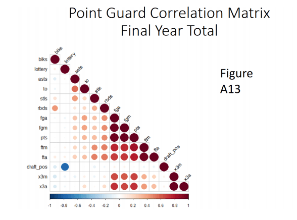
We built separate correlation matrices for Guards, Forwards, and Centers for each of the two models. Using common basketball knowledge, there was an expectation that certain statistics would be more strongly correlated to draft position for certain positions. What we found in the matrices, however, did not support that idea. For this reason, we further split the player positions into the five specific positions, breaking guards into point guards and shooting guards and also separating small forwards from power forwards. The assumption used to do this was that point guards would be identified as the shorter half of the guards while the taller half would be deemed as shooting guards. The same logic was used to determine small and power forwards. The correlation matrices were then created for each of the five positions. These are represented by the below figure.
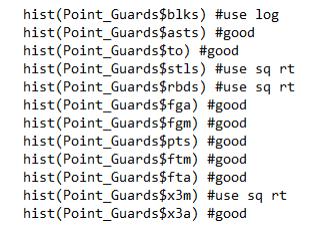
We were then ready to start the variable selection process for modeling. For each statistic, we created histograms to examine the distributions and found many to have skewness. For each variable we created a set of log-transformed statistics and square root-transformed statistics. Our variable selection process consisted of finding the most normal distribution of a statistic between the statistic itself and its two transformed versions. Once the variables were determined based on correlations and histograms, we built linear regression models with each variable as a predictor of draft position.
VIFs were calculated to examine the presence of multicollinearity. It was determined that a VIF less than three was appropriate to assume no multicollinearity existed. RMSE for each model was also calculated. The other criterion used to examine the linear regression model was to make sure that each variable in the model was statistically significant with a p-value less than 0.05. Often times, the variables in these initial models had numerous p-values over 0.05, subjecting them to removal from the models. We ran a stepwise automated selection process to let mathematics decide for us on which variables to keep and discard. This process involves tuning the regression models to keep a combination of variables with the most statistical significance and the lowest AIC for the model. If it threw out any variables that we felt that absolutely must be included in the model, we build a second regression model with the variables from the stepwise model and added back in the specific variables to be kept. RMSE was calculated for every model and models with much higher RMSEs were discarded. Upon completion of this process for each position, we cross-validated the models against average models to make sure our RMSEs were better than the average model’s RMSEs. Finally, we were ready to apply the model to the test set and compare the predictions to the actual results.
Results
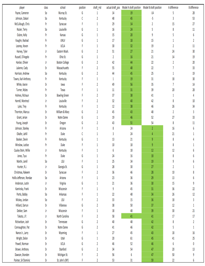
The first model based on the player’s final year of college came out with good results for the training years. All of the models based off of the five positions produced a much lower RMSE than the null model. However, when we ran these models on the test set, the results were not as good.
Let’s look at the top two and bottom two people that were expected to be drafted according to model A and see when they were actually drafted. Chris McCollough was predicted to be the highest person drafted and he was drafted 29th overall. The second highest projected pick was Jordan Mickey and he was not drafted until the second round. Delon Wright was projected to be last and he was drafted 20th. Branden Dawson did produce a more accurate model as he was supposed to be drafted near the end and was drafted 56th. The second model which was based on the career averages also produced good results in the training set, but the results in the test set were not as good. Cameron Payne had the best projected result and was drafted 14th, so that was an okay result. Dakari Johnson was the second best and he was not drafted until 48th. The two lowest projected picks were fairly accurate as Branden Dawson and Sir’Dominic Pointer were both picked late at 56th and 53rd respectively. In model B, 41 percent of the predictions were within 6 picks of the actual results, while only 26 percent met this mark for model A. However, 48 percent of the predictions in both models were within 10 picks of the actual draft results. In comparing the two models, there were no particular positions, schools, or draft classes that were predicted better from one model to the next, which would eliminate the potential too use a set of hybrid models.
Conclusion
In the end, both models produced good results on the training years while the test year predictions were hit or miss. Part of the reason for this is because a lot of prospects are drafted more on potential than how productive they are in college. Some freshmen have mediocre numbers in college, but get drafted high because of how much undeveloped talent NBA teams believe they have. For this reason, we saw the models give a much more favor to class/age. Freshmen were predicted to be drafted the highest and each subsequent year of classmen were predicted to be drafted lower. Another reason for the mediocre test results could be explained because they were tested over just one draft year. It could be possible that if we had more draft years to test on, the results could have been different, for better or for worse. Other factors that could be considered in impacting draft order for NCAA players are NBA combine results and performance in the NCAA tournament.
Great looking website. Think you did a bunch of your own html coding.
I am regular reader, how are you everybody? This post posted at this website is truly
good.
Great post. I am facing some of these issues as well..
Good day! Do you use Twitter? I’d like to follow you if that would be ok.
I’m absolutely enjoying your blog and look forward to new
updates.