

Monte Carlo simulation has many practical purposes. In finance, this approach is used to evaluate risk. In sports, we can use this same methodology to evaluate the win probability of teams or bets. In general, simulation is a great approach that approximates reality through controlled randomness.
At the most basic level, a simulation is just repeatedly sampling from a random distribution. If we sample enough, we won’t get anything new, we just re-create the old distribution. On the other hand, when we sample randomly from multiple distributions, we can approximate the interaction of events in a new distribution.
In this article we will walk through a simple way to simulate NBA games. We will be using team points scored and team points scored against to evaluate win probability. As a case study, we will simulate the 2017–2018 NBA finals to determine the expected win probability of each team.
Understanding the Data
We will be using the NBA Game Stats from 2014–2018 data set on kaggle.com. You can find this and the github link here:
For this analysis, we will need the following packages:
import pandas as pd
#Lets us read in the and manipulate the data import random as rnd
#Needed for the "random" part of simulation import matplotlib.pyplot as plt
#Allows us to visualize our results
Our first step will be to load in the data and look at the columns
gdf = pd.read_csv('nba_games_stats.csv')
gdf.columns
Based on the column output, we will only need to focus on a few variables: Team, Date, TeamPoints, and Opponent Points.
Index(['Unnamed: 0', 'Team', 'Game', 'Date', 'Home', 'Opponent', 'WINorLOSS','TeamPoints', 'OpponentPoints', 'FieldGoals', 'FieldGoalsAttempted','FieldGoals.', 'X3PointShots', 'X3PointShotsAttempted', 'X3PointShots.','FreeThrows', 'FreeThrowsAttempted', 'FreeThrows.', 'OffRebounds','TotalRebounds', 'Assists', 'Steals', 'Blocks', 'Turnovers','TotalFouls', 'Opp.FieldGoals', 'Opp.FieldGoalsAttempted','Opp.FieldGoals.', 'Opp.3PointShots', 'Opp.3PointShotsAttempted','Opp.3PointShots.', 'Opp.FreeThrows', 'Opp.FreeThrowsAttempted','Opp.FreeThrows.', 'Opp.OffRebounds', 'Opp.TotalRebounds','Opp.Assists', 'Opp.Steals', 'Opp.Blocks', 'Opp.Turnovers','Opp.TotalFouls'],dtype='object')
Next, we separate the teams we are looking at (Golden State & Cleveland) and trim the data set so that it only includes the 2017–2018 season but not the finals.
gswdf = gdf[gdf.Team == 'GSW']
cldf = gdf[gdf.Team == 'CLE']gswdf.Date = gswdf.Date.apply(lambda x: pd.to_datetime(x, format='%Y-%m-%d', errors='ignore'))gswdf = gswdf[(gswdf['Date'] > pd.to_datetime('20171001', format='%Y%m%d', errors='ignore')) & (gswdf['Date'] <= pd.to_datetime('20180531', format='%Y%m%d', errors='ignore'))]cldf.Date = cldf.Date.apply(lambda x: pd.to_datetime(x, format='%Y-%m-%d', errors='ignore'))cldf = cldf[(cldf['Date'] > pd.to_datetime('20171001', format='%Y%m%d', errors='ignore'))& (cldf['Date'] <= pd.to_datetime('20180531', format='%Y%m%d', errors='ignore'))]
With these trimmed data frames, we want to look at the distribution of points scored by and against both teams. We will use these to simulate the outcomes of the finals game.
#creates histograms of games (blue is GSW & orange is CLE)#points scored (run this first)
gswdf.TeamPoints.hist()
cldf.TeamPoints.hist()#points scored against (run this second)
gswdf.OpponentPoints.hist()
cldf.OpponentPoints.hist()
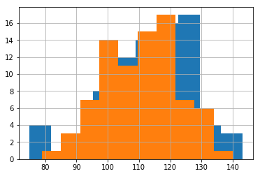
As you can see, these images fit close to a normal distribution.
For points scored, it looks like Golden State has a slightly higher average score but also a slightly more spread out point distribution than Cleveland.
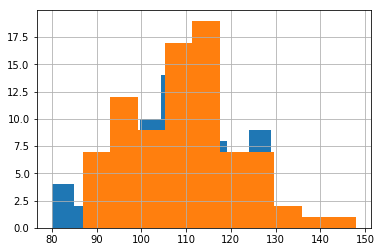
For points against, we see a similar pattern; however, it looks like the teams are closer in comparison.
In order to simulate we have to better understand these distributions. If they are normally distributed, we can re-create them based on just their mean and standard deviation.
Running the Simulation
As mentioned above, the only things that we will need to actually run the simulation are the means and standard deviations of the points scored and points scored against. We can calculate and see these here:
gswmeanpts = gswdf.TeamPoints.mean()
clmeanpts = cldf.TeamPoints.mean()
gswsdpts = gswdf.TeamPoints.std()
clsdpts = cldf.TeamPoints.std()gswmeanopp = gswdf.OpponentPoints.mean()
clmeanopp = cldf.OpponentPoints.mean()
gswsdopp = gswdf.OpponentPoints.std()
clsdopp = cldf.OpponentPoints.std()print("Golden State Points Mean ", gswmeanpts)
print("Golden State Points SD ", gswsdpts)
print("Cleveland Points Mean ", clmeanpts)
print("Cleveland Points SD ", clsdpts)print("Golden State OppPoints Mean ", gswmeanopp)
print("Golden State OppPoints SD ", gswsdopp)
print("Cleveland OppPoints Mean ", clmeanopp)
print("Cleveland OppPoints SD ", clsdopp)
We see precisely what the above distributions showed us:
Golden State Points Mean  113.46341463414635
Golden State Points SD  14.121339356922327
Cleveland Points Mean  110.85365853658537
Cleveland Points SD  12.02068377014038
Golden State OppPoints Mean  107.48780487804878
Golden State OppPoints SD  11.858469809931732
Cleveland OppPoints Mean  109.92682926829268
Cleveland OppPoints SD  12.052130069205973
The next step is to build the distributions and to start randomly sampling from them. We use the gaussian (gauss) function from the random module. This function uses a mean and a standard deviation to create a normal distribution. It then takes a random sample from that distribution and produces a value.
#randomly samples from a distribution with a mean=100 and a SD=15
random.gauss(100, 15)
For each team, we will project their score by taking a sample from their points scored distribution and the points scored against the opponent’s distribution. We will average these two numbers. We will keep doing this until our distribution reaches a limit or a satisfactory level of confidence.
Example
GSW(Score sample) + CLE(Score against sample) /2 = Projected GSW score
CLE(Score sample) + GSW(Score against sample)/2 = Projected CLE score
If Projected GSW score > Projected CLE score, then we say that Golden state won that game. We repeat this randomized process until the win % stabilizes
We write a function to take these samples from both teams and return the winner.
def gameSim():
    GSWScore = (rnd.gauss(gswmeanpts,gswsdpts)+rnd.gauss(clmeanopp,clsdopp))/2
    CLScore = (rnd.gauss(clmeanpts,clsdpts)+rnd.gauss(gswmeanopp,gswsdopp))/2
    if int(round(GSWScore)) > int(round(CLScore)):
        return 1
    elif int(round(GSWScore)) < int(round(CLScore)):
        return -1
    else: return 0
Once we have this, we create a wrapper function that lets you choose how many times to repeat this process. It also tabulates the results.
def gamesSim(ns):
    gamesout = []
    team1win = 0
    team2win = 0
    tie = 0
    for i in range(ns):
        gm = gameSim()
        gamesout.append(gm)
        if gm == 1:
            team1win +=1
        elif gm == -1:
            team2win +=1
        else: tie +=1
    print('GSW Win ', team1win/(team1win+team2win+tie),'%')
    print('CLE Win ', team2win/(team1win+team2win+tie),'%')
    print('Tie ', tie/(team1win+team2win+tie), '%')
    return gamesout
Finally, we actually simulate the results by running the function:
gamesSim(10000)
After running this 1000 times, our model projects that Golden State would win an individual game against Cleveland 57% of the time.
Output:
GSW Win  0.5669 %
CLE Win  0.4018 %
Tie  0.0313 %#I know ties can't exist in this scenario
What’s Next?
This simulation model is extremely simple and only scratches the surface of what is possible. If you want to take this analysis a step further, you can simulate games based on individual player performance rather than historic team performance. In theory, with this method, you would be able to somewhat approximate team performance when a player rests or is injured.
If you’re interested in wagering, this methodology is great because it gives you a very clear probability distribution (confidence interval). For example, from the distribution of results, we can evaluate the chances that a team expects to hit the over relative to the inferred betting odds. If your model has a higher expectation than the inferred odds, you should usually take the bet (assuming your model is good).
To make this easier, I also built a script that lets you run this analysis for any team. You can find here.
I have read so many articles or reviews concerning the blogger lovers except this article is truly a fastidious piece of writing, keep it up.| а
Thanks for the read!